This question is ambiguously defined. Electrical field lines (as referenced in the title) are not the same as equipotential lines. Specifically the electric field E followed by electric field lines is related to the electric potential field V by E = −∇V.
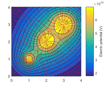
In the case of electrical potential, this is a scalar field so equipotential lines are simply contours of constant value of that field. contourf is therefore an ideal choice to visualise this.
As for field lines, quiver will show you the size and direction of vectors in the electric field, but not the field lines. The easiest way to display these in a 2D plane is streamslice.
Calculating and plotting these fields in MATLAB is just a case of setting up the physical equations in a vectorised form and calculating them for a grid of coordinates through which MATLAB can draw contours and field lines.
Using the equation for electrical potential in the form used by rwong's link in the comments above:
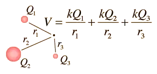
k = 8.987E9; % Coulomb's constant
p = [1,1; 2,2; 3,3];
Q = [1; 2; 3];
[X,Y] = meshgrid(0:0.05:4); % Create a grid of coordinates where V is to be calculated

V = zeros(size(X)); % Start with zero electric potential
for ii = 1:numel(Q) % Superpose the electric potential field of each charge
    V = V + k * Q(ii) ./ hypot(p(ii,1)-X, p(ii,2)-Y);
end

hContour = contourf(X,Y,V);
hColorbar = colorbar;
ylabel(hColorbar,'Electric potential (V)')
The default contour spacing will be very tightly packed around the point charges due to the singularities in electrical potential they create. If you have the Statistics Toolbox, you can quickly improve on this by finding contour levels with equal area between them using quantile:
hContour.LevelList = [0 quantile(V(:),10)];
The electric field is simpler to derive from the existing potential field than it is from the raw vector equation:
[Ex,Ey] = -gradient(V);
validColumns = all(isfinite(Ex) & isfinite(Ey)); % Ignore columns where E contains infinite values due to the point charges since streamslice can't handle them
hold on
hLines = streamslice(X(:,validColumns),Y(:,validColumns),Ex(:,validColumns),Ey(:,validColumns));
set(hLines,'Color','r');