I am simulating D flip flop in cadence, how to find set up and hold time in d FF?
And I have design negative D FF using Pass gate and Inverter when i change same circuit to positive D FF by changing ck to invClk and invclk to clk.
invclk=not(clk)
I am simulating D flip flop in cadence, how to find set up and hold time in d FF?
And I have design negative D FF using Pass gate and Inverter when i change same circuit to positive D FF by changing ck to invClk and invclk to clk.
invclk=not(clk)
Looking for the values of setup time that cause the FF to "fail to operate" is not a good idea. A FF will malfunction long before it starts to completely fail. This is a very optimistic specification for setup time, and it can lead to erroneous estimates of MTBF for metastability.
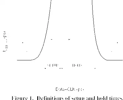
The effect of setup time on clock-to-Q delay is well known and has been documented for several kinds of flip-flops. Here's an example from 1996:
Foley, C., "Characterizing metastability," Symposium on Advanced Research in Asynchronous Circuits and Systems, 1996., pp.175,184, 18-21 Mar 1996, doi: 10.1109/ASYNC.1996.494449
Here's another example from 2001, regarding a \$0.25\mu m\$ process. In this figure you can see that the measured setup time is 190ps, allowing a 5% increase in clock-to-Q delay. If instead the setup time was estimated to be the smallest value that allows the flip-flop to operate the authors would have selected a much smaller value, about 120ps. However, this would lead to invalid timing analysis because when the setup time is reduced to 120ps the actual clock-to-Q delay has increased dramatically, from an nominal value of 1060ps to 1200ps. Of course, you could choose to specify the setup time to be 1200ps for timing analysis but then you have a longer critical path and a slower clock frequency.
Dejan Markovic, Borivoje Nikolic, and Robert Brodersen. 2001. Analysis and design of low-energy flip-flops. In Proceedings of the 2001 International Symposium on Low Power Electronics and Design, pp. 52-55. doi: 10.1145/383082.383093
Similar data for a 45nm process is in "Setup Time, Hold Time and Clock-to-Q Delay Computation under Dynamic Supply Noise" by Okumura and Hashimoto, 2010. In "Multi-Corner, Energy-Delay Optimized, NBTI-Aware Flip-Flop Design" (Abrishami, Hatami, and Pedram in 2010 ISQED) the authors present data for a 65nm process with regard to both setup and hold time. The effect of setup time on clock-to-Q delay is often discussed in the important context of metastability, such as in "Comparative Analysis and Study of Metastability on High-Performance Flip-Flops" (Li, Chuang, and Sachdev in 2010 ISQED) which again uses a 65nm process. Another example is "Performance, Metastability, and Soft-Error Robustness Trade-offs for Flip-Flops in 40nm CMOS" by Rennie et al. in IEEE Trans. on Circuits and Systems, August 2012.
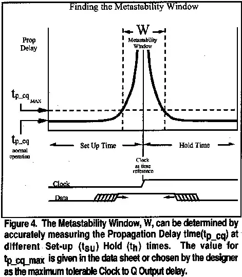
This is what I do. First, run a simulation with the D input changing one-half clock cycle before the relevant clock edge. Measure the clock-to-q delay under these conditions and consider that to be the nominal clock-to-q delay. Now start moving the D input transition closer and closer to the relevant clock edge, noticing that the clock-to-q delay will start to increase. When you have the D input edge at a point where the clock-to-q delay is 5% greater than nominal (or choose the percentage you like) then the time from D to clock is the FF setup time specification.
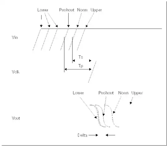
I didn't invent this technique. It is well documented in, for example, the HSPICE Applications Manual. In this manual, they refer to this effect as "pushout" of the clock-to-Q delay and state:
For setup- or hold-time optimization analysis, a normal bisection method varies the input timing to find the point just before failure. At this point, delaying the input more results in failure, and the output does not transition. In pushout analysis, instead of finding the last point just before failure, the first successful output transition is used as the golden target. You can then apply a maximum allowed pushout time to decide if the subsequent results are classified as passes or failures. Finding the optimized pushout result is similar to a normal bisection because both are using a binary search to approach the desired solution. The main difference is the goal or the optimization criteria.
The manual also supplies this figure to explain the method:
The clock-to-q delay is very sensitive to the D-to-clock time as you get close to this point so I strongly recommend using a binary search (bisection) in your simulation to find the setup time. I know this seems like a lot of work but if you do it more than once you will be glad you invested the time. Learn how to automate measurements.
For a more in-depth discussion of why this is an important criteria for defining the setup time and some SPICE simulation examples, you might also want to look at Jos Budi Sulistyo's Master's Thesis from Virginia Tech ("On the Characterization of Library Cells", 2000). Sulistyo notes that (emphasis mine):
Setup time is defined as the amount of time before the latching clock edge in which an input signal has to already reaches its expected value, so that the output signal will reach the expected logical value within a specific delay.
Deciding what is an acceptable increase in clock-to-Q (5%? 1%?) is a tricky business. Pick a small percentage and you get very conservative setup time values, which limit the maximum clock rate of your design. Pick a large percentage and you run the risk of introducing timing failures that the synthesizer can't see because it uses the nominal clock-to-q.
I interpreted your question to be specifically about running SPICE simulations to determine setup time. If instead you want to ask about the process of characterizing a standard cell flip-flop then we can talk about simulating over process corners, supply voltage, temperature, input slope, and output loading. These decisions are strongly influenced by what your synthesis tools need. For example, in an earlier life I generated characterization libraries for Synopsys' Design Compiler. There were separate libraries for different operating conditions and you included the appropriate set of libraries when performing static timing analysis. Each characterization library typically provided a 2-dimensional table for every timing parameter, showing variation due to input slope and output load. For the best results, setup and hold time should be characterized separately for a rising D input and a falling D input.
You have to skew the clock signal vs. the D input and then look through the resulting waveform for when the FF fails to operate or starts to operate again. One way is to have slightly different clock source frequencies. If your simulator allows for control over the voltage sources under Monte Carlo simulation then that is also an option. Running a complete suite of corner cases (PTV - process - temperature - voltage) especially selecting the adverse cases (Fast N slow P, or Slow P fast N) etc. and picking an appropriate sigma level in the models will then allow you to pick the appropriate delay numbers.
You'll find that the design fails very abruptly for simple logic gates transitioning over a period of a few ps so a simple sweep will be more than adequate at each PTV level.
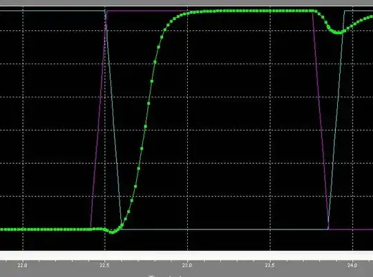
There are a couple key factors to realize. A SPICE simulation by itself is deterministic, unless you bring in foundry data and Schmoo (vary the the conditions) with foundry data your results are meaningless to determine a safe level for operational parameters. Here is a plot of a TG Based Dff with the D vs. Clk transition changing 10 ps on every 2.5 ns clock period - so a change of 0.01 ns/ 2.5 ns = 0.4% variation per clock. The high lit trace is the Output (green - Q) and you can see the circuit almost generating a runt pulse (one the RHS).
This is a very reasonable criteria to use to then do multiple runs at different PVT's. And from using the factory skewed data you can easily determine the 3 sigma level effects on the setup and hold parameters. The library industry standard is to use 3 sigma level data. More granularity (10 ps) in this case is clearly unwarranted.
Processes at or below 65 nm need to also bring in lot to lot variance ontop of mismatch to ensure that parameters are modelled and contribute accordingly.
In the following picture the two vertical red lines represent rough limits on the lengthening of Tclk-Q with the approach of the setup. The red arrows represent the span/width in this diagram. The green arrow represents the limit of the setup time (it corresponds the position of the vertical red line on the LHS. The green fuzzy band represents the statistical variation and the mismatch. With the Blue arrow representing the value that represents the safe limit of choice of Tsetup (represented by the vertical green line).
I added these features to a snip from the the other post and then added in a more realistic situation. More about that later.
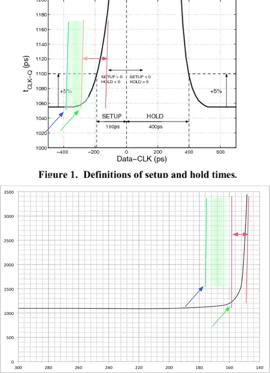
While the first image from the older paper shows this transitional area as lackadaisical event which is easily on the same scale as the setup time. For Processes that are 0.5u and below this drawing is misleading. In the simulation above, the circuit transitioned within one clock shift (in this case 10 ps) which is perhaps at most 10% of the Tsetup (0.35 um process, TG based Flip Flop). The statistical variation from process and mismatch will be many factors larger than this transitional region.
The crux of the point is that there really is no point is trying to determine this knee value when 1) it is so much more abrupt - in this case using a binary search I might have refined it to 8 ns vs. the 10 ns bin I choose. 2) this will be hidden in the noise of a value that has been choosen for yield.
I must note that in my drawing - lower part that I put in 20 ns band (red lines). Even then you can still see that the fuzzy green band will dominate.
And this drawing is for illustrative purposes only.
Is is possible, that you could have such a soft transition in this parameter. And if you do then certainly follow Joe Hass's methodology. But prepared to have that parameter smeared out with mismatch.
I do very much doubt that those are real numbers in that chart. But since I no longer have access to 1um spice decks, I cannot say, I can only suspect.
Other features. I did not do the analysis for hold as the FF's normally used have negative hold time and it would have complicated things.
I did ask around to two different groups that maintain libraries (one a library vendor one within a IDM) to make sure I wasn't screwing up.