How does negative feedback stabilize the output of an op-amp?

Question

I am trying to understand how negative feedback stabilizes the output of op-amps.

It is known that Vout = AOL*((V+)-(V-)), where AOL is the open loop gain of the op-amp, v+ is the non inverting input voltage, and v- is inverting input voltage. I took the simple case of an op-amp buffer connection so V+=vin and V-=vout.

I chose an initial value for vout=0 and ran a loop for 10 iterations with the following C code:

int main() {
    
    int Avd=100;
    int vin=1;
    float vout=0;    
    for (int i=0; i<10; i++)
    {
      vout=Avd*(vin-vout);
    }
    printf("vout %f",vout);
}

All voltages present are amplitudes of sinusoidals.

The output should reach the vin value at the end of the loop, but it reaches infinity. Why doesn't this work?

Update: I really found an excellent explanation in this question Step-by-step explanation of how voltage follower reaches steady state using negative feedback

Answer 1

How negative feedback stabilize output intuitively

It's probably best to think about an op-amp starting with a low value of \$A_{OL}\$ such as unity: -

And the big point is that the output acquires a value that completely satisfies the math and is self-sustaining. In other words, the output from the subtractor (X1) has to be 1 - 500 mV and this results in an input to the amplifier (X2) of +500 mV. It's got unity gain hence its output is also +500 mV and this self-sustains the loop.

If the gain of X2 were higher such as 10 we get this: -

So, the output is 909.91 mV and this subtracts from the 1 volt input to get 90.909 mV at the input to the amplifier (X2). Multiply 90.909 mV by ten and we get 909.09 mV at the output i.e. it is stabilized and self-sustaining.

There is a slight numerical rounding in my simulator because I'm only displaying 3 decimal places. If I choose to display 6 decimal places you'll see the "apparent" error becomes negligible: -

With a gain of 100 we get closer to the "unity-gain" situation: -

And, if we made the gain 1 million we'd see this: -

This is more like the situation with a modern and decent op-amp.

why this doesn't work

Your simulation doesn't work because it regards the op-amp as a kind-of clocked device where recalculations are performed in a sampled manner. Of course you can use this method to simulate an op-amp but you need to be much subtler.

If I simulated a similar situation to yours by adding a delay element like this: -

And, if I looked at how the output changes over time I get crazy oscillating values like this: -

Note the Y-scale is +/- 5e101 i.e. ridiculously high.

Answer 2

There are multiple factors at play here. Like most electronic circuits, the operational amplifier relies on imperfections to work. Here, it cannot output an infinite current, or alternatively, it has a limited slew rate that prevents it from changing its output too quickly. This stems from a finite output impedance, as well as a non-zero input impedance of the rest of the circuit.

Adjusted code that limits variations to 0.085V per loop (arbitrary, but below the initial delta, and deliberately cannot be added up to 1.0):

#include "stdio.h"

float max(float a, float b)
{
    return a<b?a:b;
}

float absf(float a)
{
    return a>0?a:-a;
}

float sign(float a)
{
    return a<0?-1:1;
}

int main() {
    
    int Avd=100;
    int vin=1;
    float vout=0;
    float maxdelta = 0.085;
    for(int i=0;i<15;i++)
    {
       float outth = Avd * (vin-vout); // Theoretical output
       float deltaamp = outth-vout; // How much the output should increase
       float delta;
       if ( absf(deltaamp) > maxdelta)
           delta = sign(deltaamp)*maxdelta; // max variation in the right direction
       else
           delta = deltaamp;
       vout += delta;
    printf("Theoretical increase of %f, limitted to %f, new vout=%f\n", deltaamp, delta, vout);
    }
    printf("vout %f",vout);
}

It is an imperfect model, but it will get closer to the real circuit if you imagine that loops run much faster, with a much smaller maxdelta.

As to how the output oscillations are reduced, this is also covered in that answer.

Answer 3

The rule about equilibrium

At rest (equilibrium) in op-amp circuits with negative feedback, the ratio of the op-amp output voltage to the differential input voltage is equal to its open loop gain. As the input voltage increases, the ratio decreases and the op amp starts increasing its output voltage to restore it. When this happens, the equilibrium is restored.

So the condition for achieving equilibrium in op-amp circuits with negative feedback, is the ratio of the op-amp output voltage to the differential input voltage equals its open loop gain.

This condition is violated in two cases:

• at the first moment, when the input voltage changes
• when the output voltage reaches the supply voltage

Solving the problem requires time in the first case and voltage in the second case.

Analogies

Let's now illustrate this rule with some analogous circuits - electronic and electrical.

Op-amp inverting amplifer-integrator

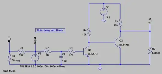
In fact, during the transition, the op-amp is temporarily an "integrator", and at the end of the transition, it becomes an amplifier again. Therefore, we can model it as a real op-amp integrator in which the capacitor C is shunted by the resistor R2.

^{simulate this circuit – Schematic created using CircuitLab}

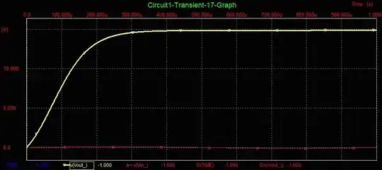
Thus, this configuration represents a very imperfect "op-amp" - single-ended, inverting and with small but fixed gain A = -R2/R1 = -10. During the transition, this amplifier is temporarily an inverting integrator, and at the end of the transition, it becomes an inverting amplifier again.

The graph below shows the calculated gain Vout/Vin which during the transition changes from zero to -10.

Voltage divider capacitively loaded

A similar but passive configuration is a voltage divider that is loaded by a capacitor.

^{simulate this circuit}

During the transition, the voltage divider is temporarily an RC integrator circuit, and at the end of the transition, it becomes a voltage divider with transfer ratio of R2/(R1 + R2) again.

The graph below shows the calculated transfer ratio Vout/Vin which during the transition changes from zero to (almost) 1.

The role of the gain

After formulating the above rule about equilibrium, I decided to turn to my favorite topic of thought, how op-amp gain affects circuit performance. This led me back to an old answer of mine where I visualized the operation of the inverting amplifier when reaching the equilibrium.

The voltage diagram

I did it using a voltage diagram that shows the voltage distribution along a resistive film. For this purpose, I replaced the discrete resistors R1 and R2 with a linear potentiometer. And now I decided to simulate this imaginary experiment with the help of CircuitLab to make it a little more real. But here a problem arose how to visualize the local voltages inside the potentiometer using the DC sweep simulation...

The new tool

A few hours ago I went out for a walk thinking about the problem... and the "new" idea came to me. It was based again on the properties of the old 19th century bridge configuration:

If we connect two linear resistors (the two bridge arms) in parallel, the opposite points of the resistive films will have the same voltages (I have come to this observation quite a long time ago sometime in my student years and have used it for other purposes). Therefore, we can connect a "measuring" ("copy") potentiometer P2 to a linear resistor or other potentiometer P1, and by moving its wiper, measure the local voltages inside the resistor (potentiometer P1). We can then run a DC sweep simulation with parameter K.P2 and observe the voltage distribution inside the potentiometer (voltage diagram). Try it!

^{simulate this circuit}

As we can see, when "moving" the P2's wiper from left to right (changing the potentiometer's transfer ratio K from 0 to 1), the voltage drop linearly decreases from 1 V to 0 V. This is the voltage diagram of P2 that is a copy of the P1's voltage diagram. So what we see in P2 is the same as in P1. In practice, we open the CircuitLab properties and start changing K from 0 to 1 while watching the voltmeter reading and then run DC sweep simulation with parameter K.P2. As a result, we see the voltage diagram below where the middle wiper's location (K = 0.5) is indicated by a thin vertical line in black and the zero voltage level - by a horizontal line in red.

Inverting amplifier investigated

Now that we can peek inside any resistor, rheostat, or potentiometer with this magical "copy potentiometer," let's perform a virtuosic experiment with our favorite inverting amplifier. In this conceptual circuit, I have used a generic op-amp, currently set to a very low open loop gain of 10x. With it, I have made an inverting amplifier with a gain of -1, "moving" the P1's wiper in the middle (its r2 = r1, K = 0.5). I have also moved the P2's wiper in the middle (its r2 = r1, K = 0.5). As a result, the voltmeter shows the voltage of the op-amp inverting input. As we can see, this voltage of 98 mV is quite different from the zero voltage of a virtual ground, i.e. there is no virtual ground.

^{simulate this circuit}

In fact, there is a virtual ground, but it has "entered" inside to the right of the P1's wiper. То find it, open the P2 properties and begin increasing K ("moving" the P2's wiper to right) until the voltmeter shows 0 V. I found that K = 0.55455.

After running the DC sweep simulation with parameter K.P2, we see that the local voltages along P1 (P2) linearly decrease from 1 V to -800 mV. Why do not they reach - 1 V?

The reason is the very small op-amp gain factor (only 10). We can figuratively imagine the voltage diagram as a kind of Archimedean "lever" - the input voltage "raises" it on the left, and the op-amp output voltage lowers it from the right. But because the op-amp has very little gain, it does not have enough power to pull it up enough, and you end up with this 98mV voltage at the midpoint of the potentiometer. Also, the circuit (inverting amplifier) gain is -0.8 instead -1.

More experiments

Now you can set a variety of gain factors (from one to several hundred thousand) and observe what the inverting input voltage (virtual ground) and the output voltage are. For example, you will see that at gains about 300,000 it is only four microvolts and the magnitude of the output voltage is exactly equal to the input voltage.

If you want to change the inverting amplifier again, "move" the P1's wiper (change K.P1 above or below 0.5).

It would also be interesting to observe the voltages when the output voltage reaches the supply voltage but this requires an op-amp with a supply.

Answer 4

The equation you’re using is only valid at DC. As soon as the time is passing in the simulation, you’re not at DC but AC, and need an AC model that includes at least first-order roll-off, since that’s what makes even ideal op-amps works at all.

So, look for how to add a roll-off in time-discrete models, and the simulation will work :)