Preface
Moses, there are two completely different perspectives about the BJT. One is the DC perspective, which helps to work out the quiescent biasing point (operating point) for the BJT. This is important because it sets the stage for the next perspective, the AC perspective, which is applied to understanding how small-scale changes are predicted/understood.
You can think of the DC perspective as the large-scale view that includes all of the non-linear behaviors of the BJT in order to find out how things settle out, once the power is applied but before any signal changes occur. And the AC perspective then tells you, once you know this DC perspective, how a tiny wiggle or change (that rides on top of the DC operating point you discovered already through non-linear mathematics) at one point in the circuit will be observed at some other point in the circuit.
These two different perspectives answer two completely different questions.
The DC perspective helps you figure out where, on some highly non-linear behavior of the BJT, the BJT is actually operating. This is like picking out a specific point on a curve. The AC perspective is a linearization (the tangent line found locally at that point on the large-scale DC curve.) It's a lot simpler to apply because it's just a simple line. But if you deviate far from it, then it gets further and further from the truth. So it is only useful for small signal changes that take place around the DC operating point.
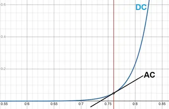
Let's look at what I mean. Here's an example chart:
To find the DC operating point, you need to use the full Ebers-Moll model. There are ways to simplify that process to get close. But exact solutions require some advanced mathematics or else a simulator. It's not necessary to use exact solutions, though, since BJTs vary so much one-to-another. So approximations usually work well.
Once the DC operating point is found (approximately or exactly), you can now take the slope at that point and greatly simplify the math involved in understanding how the BJT will behave when faced with small signals nearby this point.
To summarize:
- The blue curve is similar to the large-scale, highly non-linear behavior of a BJT and it is used to find the DC operating point.
- Once the DC operating point is uncovered by some means, then a nice tangent line (shown in black) can be drawn at this point to describe the AC behavior for small signals near the DC operating point.
One process is used to find the DC operating point. A second and different process is used to then develop and use the linear tangent line at that point for AC analysis. Your top diagram represents a schematic that might be used to find the DC operating point. Your bottom diagram represents a schematic that may be used to understand the AC behavior. These are two completely different perspectives. Both are true. But they are used for entirely different purposes.
You need to hold two things in your mind at once. Life is sometimes like that.
And keep in mind that often people will talk about the AC model as though it applies over a very long range. (Your grounded-emitter shown in the top diagram would be one-such.) But it does not. It only applies over a small range. If an input signal is large enough then the output will suffer from distortion caused by the BJT's actual non-linear behavior, which rapidly deviates from the assumed tangent line when straying too far from that assumed operating point.
So hold that third thing in mind, as well, I suppose.
Ebers-Moll
There is the DC model, which as I already mentioned is highly non-linear but it is absolutely necessary in order to work out all the voltages and currents in a circuit surrounding a BJT, when there is no signal being applied (or in circuits where there is no signal, at all.)
The earliest complete DC model was described by Ebers and Moll and didn't include AC elements nor basewidth modulation (which they assumed was constant and didn't vary.) Three different, but entirely equivalent, models were then constructed from their paper. These are the transport, the injection, and the hybrid -\$\pi\$ models. You can see all three of these equivalent models in an answer I provided here. There is NO difference in prediction between them. It's just a difference in perspective, is all.
These, collectively, can be considered the Level I Ebers-Moll model.
When charge storage (modeled as capacitance -- Level II) and basewidth modulation (discussed in a later paper by Early -- Level III) were later factored into the Ebers-Moll model, they modified only the hybrid -\$\pi\$ model. (I don't ever recall seeing a paper adding charge storage or basewidth modulation to either the injection or transport models, though I'm sure it could be done.) Charge storage is more important for the AC perspective. Basewidth modulation impacts both the DC and AC perspective.
More Simplification in Active Mode
Almost no one bothers with the Level I Ebers-Moll model, on paper at least. Instead, they simplify things still further. (If you go to the link I provided, you will see some good reasons why it's over-thinking the real need of designers.) For most purposes, the BJT is broken up into two behaviors of interest:
- Active (amplifier) mode, where the collector behaves much like a current source/sink and the base current (allowed to find it's own value and isn't specifically set by the designer) is very small compared to the collector current.
- Saturated (switch) mode, where the collector behaves a lot more like a voltage source and the base current (set within a narrow range by the designer) is much larger (than in case #1) when compared to the collector current.
In the first case, the Shockley diode equation can be used to find the relationship between the base-emitter voltage and the collector current. Keep in mind here that this works both ways. If you drive a current into the BJT's collector, you will get a base-emitter voltage as a result of that action. Or, if you drive a base-emitter voltage then you will get a collector current as a result of that action.
In the second case, the BJT is being used as a switch and it's not really a part of your question. So I'll avoid further discussion about it.
In active mode, a simplified relationship can be expressed by the Shockley equation, as modified here:
$$I_{_\text{C}}=I_{_\text{SAT}}\cdot\left[\exp\left(\frac{V_{_\text{BE}}}{\eta\,V_T}\right)-1\right]$$
This is the highly non-linear, large-scale model equation for active mode. It can be used to help find the DC operating point.
This can be turned around to get this:
$$V_{_\text{BE}}=\eta\,V_T\cdot\ln\left[1+\frac{I_{_\text{C}}}{I_{_\text{SAT}}}\right]$$
The value of \$I_{_\text{SAT}}\$ and the emission coefficient (ideality factor, etc) \$\eta\$ are model parameters. They are assumed or given and taken as constants. (They aren't constant -- and especially \$I_{_\text{SAT}}\$ is highly temperature-dependent.) Usually, \$\eta=1\$ is taken as granted for small signal BJTs. But you should be warned that this isn't usually the case for power BJTs. Regardless, these are model parameters.
There's another model parameter, \$\beta\$, which is the ratio of collector current to base current. It's also often taken to be constant (but not known very precisely.)
For AC analysis, we need to take the derivative of these equations to find the tangent line. This leads to concepts such as \$r_e^{\,'}=\frac{V_T}{\vert\,I_{_\text{E}}\,\vert}\$ and \$r_\pi\$, which are not actual resistances but instead the rate of change of voltage divided by the rate of change of current, which is kind of a so-called dynamic resistance. (Or \$g_m\$ which is inversely related.) Instead, they all in some way represent that black line I drew on the picture above. And they are used for AC analysis. Not for DC operating point analysis.
Summary
Hopefully, all this gets across the fact that there are two very different, but equally important, areas of analysis when looking at a BJT subcircuit. One is to first find (or set) its DC operating point. The other is to find (or set) it's AC amplification behavior. These are two completely different needs by a designer and there are two completely different processes used, as well.
You may have conflated them in your question. Hopefully, the above helps you to separate them back out, again, so that you see them as two distinct concepts used for two different purposes.


