Initial Answer
I won't perform the solution (yet.) But I can suggest a process for analyzing the circuit when the base currents aren't assumed to be zero.
Let's look at the annotated schematic:
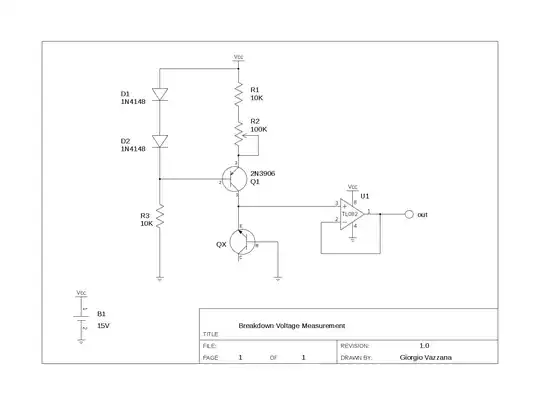
simulate this circuit – Schematic created using CircuitLab
Before I begin, just a few notes about the above schematic:
- I'm assuming that both BJTs will be in their active mode. If, for any reason, your analysis finds that either one of them is not in active mode then what I present here fails. This is a normal way to proceed, though. Start with this assumption, perform the calculations, apply them to the schematic and see if the results confirm the assumption.
- There are two base-emitter voltages indicated in the schematic. But, for analysis, you don't actually need the one for \$Q_2\$. (Except when testing to see if the results confirm the assumptions in #1 above.)
- You will need the base-emitter voltage for \$Q_1\$. You can either supply it as an assumption you make or, if you want a closed solution, you can develop it using the Shockley diode equation. However, I don't recommend going that direction as it requires you to have some experience with one of the branches of the product-log function (LambertW) and that's unlikely unless you study mathematics outside the typical undergrad curriculum.
- You will have to supply some assumed values for \$\beta_1\$ and \$\beta_2\$ for their respective BJTs.
You can apply KCL to nodes \$V_1\$ and \$V_2\$. That should be pretty easy to lay out. You can apply KVL to two loops: (1) From \$V_{_{\text{CC}}}\$, through \$R_{_{\text{B}_3}}\$, through \$R_{_{\text{B}_2}}\$, via \$V_{_{\text{BE}_1}}\$, then finally through \$R_{_{\text{E}}}\$. (2) From \$V_{_{\text{CC}}}\$, through \$R_{_{\text{B}_3}}\$, through \$R_{_{\text{B}_2}}\$, then finally through \$R_{_{\text{B}_1}}\$.
You should carefully note that there are clear, definite relationships between a number of the unknowns shown in the schematic. Two of these unknowns that you will need to find directly are obviously \$V_1\$ and \$V_2\$. But you can select exactly two currents as your additional unknowns to find and then take note of the quantitative relationships that all the remaining currents have to these two. I'd recommend that one of the currents should be either of the two base currents, with the other one pretty much any one of the five resistor currents.
After substitutions, this provides four equations in four unknowns and it is easily solvable.
Added for Autodidacts
A day's gone by, now. And I may as well work through the problem (before I move on in life) for those interested in seeing how a solution may develop from the above discussion.
This is added for those kindred self-educators.
Let's first re-state the schematic with some added information. We'll need this when developing the equations.
simulate this circuit
Be sure to carefully trace out the additions I've added above. As you may well see, now all of the currents are dependent upon exactly two unknown currents, \$I_{_{\text{B}_1}}\$ and \$I_{\text{R}_{\text{B}_1}}\$. With that in hand, the KVL equations can be developed shortly.
But first, the easiest part is the KCL for the nodes associated with \$V_1\$ and \$V_2\$.
$$\begin{align*}
\frac{V_1}{R_{_{\text{B}_1}}}+\frac{V_1}{R_{_{\text{B}_2}}} +I_{_{\text{B}_1}} &=\frac{V_2}{R_{_{\text{B}_2}}}
\\\\
\frac{V_2}{R_{_{\text{B}_2}}}+\frac{V_2}{R_{_{\text{B}_3}}}+\left(I_{_{\text{B}_2}}=I_{_{\text{B}_1}}\cdot\frac{\beta_1}{\beta_2+1}\right) &=\frac{V_1}{R_{_{\text{B}_2}}}+\frac{V_{_{\text{CC}}}}{R_{_{\text{B}_3}}}
\end{align*}$$
I've used a technique above that I've developed (and discuss in the KCL
Addendum below) for quickly and accurately writing out the particular form of the above
equations. The results are exactly the same as other forms.
I just prefer these. I've found I make far
fewer mistakes that way. But feel free to re-arrange the above equations
into any form that feels more comfortable. They will be
mathematically equivalent, as you'll see if you try it.
The above two equations have three unknowns: \$V_1\$, \$V_2\$, and \$I_{_{\text{B}_1}}\$.
The KVL below follows through with my earlier discussion and in the order I listed them:
$$\begin{align*}
V_{_{\text{CC}}} - R_{_{\text{B}_3}}\cdot I_{\text{R}_{\text{B}_3}} - R_{_{\text{B}_2}}\cdot I_{\text{R}_{\text{B}_2}} - V_{_{\text{BE}_1}} - R_{_{\text{E}}}\cdot I_{_{\text{E}_1}} &= 0\:\text{V}
\\\\
V_{_{\text{CC}}} - R_{_{\text{B}_3}}\cdot I_{\text{R}_{\text{B}_3}} - R_{_{\text{B}_2}}\cdot I_{\text{R}_{\text{B}_2}} - R_{_{\text{B}_1}}\cdot I_{_{\text{B}_1}} &= 0\:\text{V}
\end{align*}$$
Using the annotations in the latest schematic above we can make some substitutions and reduce the unknowns:
$$\begin{align*}
V_{_{\text{CC}}} - R_{_{\text{B}_3}}\cdot \left(I_{\text{R}_{\text{B}_1}}+I_{_{\text{B}_1}}\!\!\left[1+\frac{\beta_1}{\beta_2+1}\right]\right) - R_{_{\text{B}_2}}\cdot \left(I_{\text{R}_{\text{B}_1}}+I_{_{\text{B}_1}}\right) - V_{_{\text{BE}_1}} - R_{_{\text{E}}}\cdot I_{_{\text{B}_1}}\cdot\left(\beta_1+1\right) &= 0\:\text{V}
\\\\
V_{_{\text{CC}}} - R_{_{\text{B}_3}}\cdot \left(I_{\text{R}_{\text{B}_1}}+I_{_{\text{B}_1}}\!\!\left[1+\frac{\beta_1}{\beta_2+1}\right]\right) - R_{_{\text{B}_2}}\cdot \left(I_{\text{R}_{\text{B}_1}}+I_{_{\text{B}_1}}\right) - R_{_{\text{B}_1}}\cdot I_{\text{R}_{\text{B}_1}} &= 0\:\text{V}
\end{align*}$$
This only adds one more unknown: \$I_{\text{R}_{\text{B}_1}}\$.
So now there are just four unknowns and four equations to solve. Using the freely available SymPy:
eq1 = Eq( v1/rb1 + v1/rb2 + ib1, v2/rb2 )
eq2 = Eq( v2/rb2 + v2/rb3 + ib1*beta_1/(beta_2+1), v1/rb2 + vcc/rb3 )
eq3 = Eq( vcc - rb3*(irb1+ib1*(1+beta_1/(beta_2+1))) - rb2*(irb1+ib1) - vbe - re*ib1*(beta_1+1), 0 )
eq4 = Eq( vcc - rb3*(irb1+ib1*(1+beta_1/(beta_2+1))) - rb2*(irb1+ib1) - rb1*irb1, 0 )
ans = solve( [ eq1, eq2, eq3, eq4 ], [ v1, v2, ib1, irb1 ] )
This is a symbolic solution, not numerical. So to get numerical results we will need to specify numerical inputs for each known variable.
To achieve this, I need a starting place to generate values for the circuit.
Here are some assumptions I'll use:
- Quiescent \$I_{_{\text{E}_1}}=1\:\text{mA}\$.
- \$R_{_{\text{E}}}=1\:\text{k}\Omega\$ to set \$V_{_{\text{E}_1}}=1\:\text{V}\$.
- \$V_{_{\text{BE}_1}}=660\:\text{mV}\$ @ \$I_{_{\text{E}_1}}=1\:\text{mA}\$.
- \$Q_1\$ is LTspice model for 2N3904, except \$\beta_1=150\$.
- \$Q_2\$ is LTspice model for 2N3904, except \$\beta_2=250\$.
- Biasing stiffness: \$I_{\text{R}_{\text{B}_1}}\approx 100\:\mu\text{A}\$.
- \$R_{_{\text{C}}}=4.7\:\text{k}\Omega\$ (some modest voltage gain.)
- \$V_{_{\text{CC}}}=15\:\text{V}\$.
From the above, add this:
- Quiescent \$V_{_{\text{C}_2}}\approx V_{_{\text{CC}}}-R_{_{\text{C}}}\cdot I_{_{\text{E}_1}} = 10.3\:\text{V}\$. Allowing room for \$\pm 2\:\text{V}\$ swing, this means as low as about \$8\:\text{V}\$, when active. I like another \$2\:\text{V}\$ of margin to keep \$Q_2\$ well out of saturation, so I'll assign \$V_2=6\:\text{V}\$ as a design goal.
Now I can compute the rest:
- \$V_1=V_{_{\text{E}_1}}+V_{_{\text{BE}_1}}=1\:\text{V}+660\:\text{mV}=1.66\:\text{V}\$
- \$I_{_{\text{B}_1}}=\frac{1}{\beta_1+1}\cdot I_{_{\text{E}_1}}=\frac{1\:\text{mA}}{150+1}\approx 6.6\:\mu\text{A}\$
- \$I_{_{\text{B}_2}}=\frac{\beta_1}{\beta_1+1}\cdot \frac{1}{\beta_2+1}\cdot I_{_{\text{E}_1}}\approx 4.0\:\mu\text{A}\$
- \$I_{\text{R}_{\text{B}_2}}=I_{\text{R}_{\text{B}_1}}+I_{_{\text{B}_1}}\approx 107\:\mu\text{A}\$
- \$I_{\text{R}_{\text{B}_3}}=I_{\text{R}_{\text{B}_2}}+I_{_{\text{B}_2}}\approx 111\:\mu\text{A}\$
- \$R_{_{\text{B}_1}}=\frac{V_1}{I_{\text{R}_{\text{B}_1}}}=\frac{1.66\:\text{V}}{100\:\mu\text{A}}=16.6\:\text{k}\Omega\$
- \$R_{_{\text{B}_2}}=\frac{V_2-V_1}{I_{\text{R}_{\text{B}_2}}}=\frac{1\:\text{V}+660\:\text{mV}}{107\:\mu\text{A}}\approx 41\:\text{k}\Omega\$
- \$R_{_{\text{B}_3}}=\frac{V_{_{\text{CC}}}-V_2}{I_{\text{R}_{\text{B}_3}}}=\frac{15\:\text{V}-6\:\text{V}}{111\:\mu\text{A}}\approx 81\:\text{k}\Omega\$
I'll round the resistor values using E24 series values.
simulate this circuit
Now to make predictions using SymPy's solution:
for y in ans:
    y, ans[y].subs({rb1:18e3,rb2:39e3,rb3:82e3,vbe:.66,beta_1:150,beta_2:250,vcc:15,re:1e3})
(v1, 1.77926399160283)
(v2, 5.92341740170372)
(ib1, 7.41234431525051e-6)
(irb1, 9.88479995334904e-5)
And finally, to now run LTspice:
In good agreement.
As another double-check, both BJTs are in active mode according to LTspice. I'd designed it that way. But it's nice to see that the design didn't go astray from my intent.
Let's now flip the \$\beta\$ values for the two BJTs and see if SymPy's results still match the modified LTspice run. The circuit wasn't designed using those values. But it should survive the run, I think.
SymPy says:
for y in ans:
    y, ans[y].subs({rb1:18e3,rb2:39e3,rb3:82e3,vbe:.66,beta_1:250,beta_2:150,vcc:15,re:1e3})
(v1, 1.79243375213728)
(v2, 5.85199605706693)
(ib1, 4.51168825552700e-6)
(irb1, 9.95796528965154e-5)
LTspice says:
Again, looks reasonably close.
We could also change resistor values and so on. But I think there's some confidence already that the analysis was soundly reasoned.
Some final notes about the above.
We made an assumption (and I got lucky) about the base-emitter voltage of \$Q_1\$. LTspice didn't make that assumption. It uses a fairly detailed model and an iterative process in order to compute it. Far beyond what we are likely to ever manage without such a program to help.
However, we can use a tool like LTspice to inform us better, in simulation, and we can then use that better value in our manual computations to verify that we'd get still closer. That's a additional small test about our thinking processes that could be made. But we've already many other ways of testing ourselves (such as changing the \$\beta\$ values as done once above, for example, to see if our analytical result continues to stay close to SPICE computations.)
Also, SPICE should be used to help confirm your analytical thinking. It should not be a source of 'hunt-and-peck' design, where you keep plugging in values hoping that something useful comes out in the end. You don't evolve a circuit through mutation and selection. That's a different subject called evolutionary biology. Not electronics design. You should have enough of the process to follow that SPICE tends to confirm your thinking.
KCL Addendum
The KCL equations may appear to treat node voltages as if they don't have to be differences, but can be absolute values. However, that's not really the case here. In fact, I'm just using superposition (which is easily seen once you've really had the concepts deepened into you.) This is, in fact, the same technique used within Spice programs (those where I've directly looked over the code used to generate these.)
Perhaps the easiest way to imagine is that absolute voltage at a node spills away from that node through the available paths. But also that absolute voltages spill into that node from surrounding nodes through those same paths. So long as you treat them all as absolute values, the result is the application of a simple superposition concept that results in, effectively, the potential differences controlling the result.
You can test this, easily, by rearranging the resulting equation(s), moving the right side over to the left side and then combining terms. You'll then see the usual potential differences that you expect. So it really is the same result.
The reason I very much prefer this method is that it is simple to visualize and very difficult to make mistakes. You can easily orient yourself to a node and then work out the terms for out-flowing currents for the left side of the equation. Then all you have to do is position yourself at each surrounding node and work out the terms for in-flowing currents for the right side. It's almost impossible to screw that up.
Conversely, when you are instead struggling to work out the potential differences in your mind (using the more traditionally taught method) and just write those terms, you often find yourself not entirely sure if you have the sign right as you try and add them up, correctly. I find, time and time again that not only others wind up messing up somewhere and making an uncaught mistake.. but that I also make those mistakes, as well. Even with lots of experience, you just aren't 100% sure and you often find yourself double and triple checking your work, just in case.
That doesn't ever happen, once you start using the superposition method. It just works. It just works right. It just works right each and every time. I've never, not once, screwed up. (I make typos. But not sign errors.) It's too easy to use.
So voltage spills away from a node via available paths and voltage spills into a node from nearby nodes via the same available paths. The only caveat is that a current source or sink can only flow in, or flow out, but not both directions. It's one way. So it will either appear on the out-flowing side or on the in-flowing side -- but not both sides.
This also works perfectly well with capacitors and inductors. It does turn the equation into a differential/integral equation. But that's just a technicality. It's still correct.

