On the huge error between LTSPICE and Ebers-Moll when vCE=0 for a BJT

Question

1. Let us assume that we have a npn BJT with parameters similar to 2N2222 in LTSPICE at T=27 C
2. The thermal voltage at T=27C is VT=25.865 mV
3. Let us assume that VCE=0 and VBE=0.85 V
4. From 2N2222 in LTSPICE we have: IS=10^-14 A, VA=100 V, BETA=200, BR=3
5. From Ebers-Moll equation we get: IC=IS[EXP(VBE/VT)-EXP(VBC/VT)](1-VBC/VA)-IS BR^-1* (EXP(VBC/VT)-1)
6. Since VCE=0, VBE=VBC, then Ebers-Moll will be simplified as: IC=-IS *BR^-1 *(EXP(VBE/VT)-1)=-10^-14 *3^-1 *[EXP(850/25.865)-1]=-0.6 A
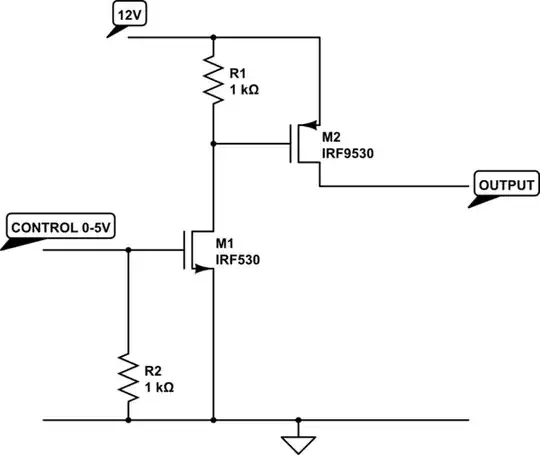
7. If you use LTSPICE as below you get IC=-0.008 A which is a huge error compared to Ebers-Moll (-0.6 A), Do you know what causes this huge error?

Answer 1

The following model doesn't show many of the physical details, but it at least shows you where the simplified Ebers Moll Level I model applies and where the Level II bulk impedances go:

^{simulate this circuit – Schematic created using CircuitLab}

LTspice cannot show you the internal values within the BJT that are shown primed in the above diagram. All it can do is show you the external voltages that you've applied and what it works out as the currents through the voltage sources I've added to the diagram.

A BJT is asymmetrical. The collector is only lightly doped and by comparison the emitter is more heavily doped. The internal collector voltage, \$V_{_\text{C}}^{'}\$, despite externally grounded in your diagram, must always (because of the relative doping) find a voltage in between that of \$V_{_\text{E}}^{'}\$ and \$V_{_\text{B}}^{'}\$. It cannot be below \$V_{_\text{E}}^{'}\$.

Because of the relatively small value for \$R_{_\text{C}}^{'}\$, even a very small \$V_{_\text{CE}}^{'}=V_{_\text{C}}^{'}-V_{_\text{E}}^{'}\$ will mean a much larger (out-flowing in this case) collector current than an (out-flowing) emitter current (The base supplying both, obviously.)

The model used by LTspice for the 2N2222 is: IS=1E-14, VAF=100, BF=200, IKF=0.3, XTB=1.5, BR=3, CJC=8E-12, CJE=25E-12, TR=100E-9, TF=400E-12, ITF=1, VTF=2, and XTF=3. Unspecified explicitly, but defaulted are: NF=1, NE=1.5, NC=2, MJE=.33, MJC=.33, VJC=.75, VJS=.75, XTI=3, VG=1.206, VO=10, etc. In short, there are quite a few parameters (many that you've not taken into consideration) that relate to Spice's initial DC operating point computations.

But let's keep it simple and just use the Ebers Moll Level I model, and the above slightly modified (not quite Level II) version of events. And let's accept the assumption I earlier mentioned, that LTspice is getting things right enough that we can estimate a few details in the above model (as shown with labels there.)

Keep in mind that I'm only grossly estimating and rounding the values. So we have the following as starting points:

• \$V_{_\text{B}}^{'}\approx 750\:\text{mV}\$

  (\$850\:\text{mV}-10\:\Omega\cdot 10.394\:\text{mA}\approx 746\:\text{mV}\$, then rounded)

• \$V_{_\text{E}}^{'}\approx 500\:\mu\text{V}\$

  (\$200\:\text{m}\Omega\cdot 2.33343\:\text{mA}\approx 467\:\mu\text{V}\$, then rounded)

• \$V_{_\text{C}}^{'}\approx 2.5\:\text{mV}\$

  (\$300\:\text{m}\Omega\cdot 8.05797\:\text{mA}\approx 2.42\:\text{mV}\$, then rounded)

• \$V_T=25.865\:\text{mV}\$ (your calculation)

And here are the equations from the non-linear hybrid-\$\pi\$ model that I show here:

• \$\frac{I_{_\text{CC}}}{\beta_{_\text{F}}} = \frac{I_{_\text{S}}}{\beta_{_\text{F}}} \cdot \left[ e^{\frac{q\cdot V_{_\text{BE}}}{k\cdot T}} - 1 \right] \$
• \$\frac{I_{_\text{EC}}}{\beta_{_\text{R}}} = \frac{I_{_\text{S}}}{\beta_{_\text{R}}} \cdot \left[ e^{\frac{q\cdot V_{_\text{BC}}}{k\cdot T}} - 1 \right] \$
• \$I_{_\text{CT}} = I_{_\text{CC}} - I_{_\text{EC}}, \rm{(generator \,\, current)}\$
• \$ I_{_\text{C}} = \left( I_{_\text{CC}} - I_{_\text{EC}} \right) - \frac{I_{_\text{EC}}}{\beta_{_\text{R}}} \$
• \$ I_{_\text{B}} = \frac{I_{_\text{CC}}}{\beta_{_\text{F}}} + \frac{I_{_\text{EC}}}{\beta_{_\text{R}}} \$
• \$ I_{_\text{E}} = -\frac{I_{_\text{CC}}}{\beta_{_\text{F}}} - \left( I_{_\text{CC}} - I_{_\text{EC}} \right) \$

Let's just compute those in order:

1. \$\frac{I_{_\text{CC}}}{\beta_{_\text{F}}} = \frac{10\:\text{fA}}{200} \cdot \left[ e^{\frac{750\:\text{mV}-500\:\mu\text{mV}}{25.865\:\text{mV}}} - 1 \right]= 192.17078\:\mu\text{A}\therefore I_{_\text{CC}}=38.4341559\:\text{mA}\$

2. \$\frac{I_{_\text{EC}}}{\beta_{_\text{R}}} = \frac{10\:\text{fA}}{3} \cdot \left[ e^{\frac{750\:\text{mV}-2.5\:\text{mV}}{25.865\:\text{mV}}} - 1 \right]= 11.8580823\:\text{mA}\therefore I_{_\text{EC}}=35.5742468\:\text{mA} \$

3. \$I_{_\text{CT}} = 38.4341559\:\text{mA} - 35.5742468\:\text{mA} = 2.8599091\:\text{mA}\$

4. \$ I_{_\text{C}} = 2.8599091\:\text{mA} - 11.8580823\:\text{mA} = -8.9981732\:\text{mA}\$

   (LTspice says: \$ -8.05797\:\text{mA}\$)

5. \$ I_{_\text{B}} = 192.17078\:\mu\text{A} + 11.8580823\:\text{mA} = 12.050253\:\text{mA}\$

   (LTspice says: \$10.3914\:\text{mA}\$)

6. \$ I_{_\text{E}} = -192.17078\:\mu\text{A} - 2.8599091\:\text{mA} = -3.05207988\:\text{mA}\$

   (LTspice says: \$-2.33343\:\text{mA}\$)

Even the meager Ebers-Moll Level I model (with internal bulk resistances added, aka Level II) gets kind of close, using values I rounded. (I'll demonstrate in a minute what it means if I used values closer to what LTspice had to work with.)

It doesn't take into account the fuller, adapted Gummel-Poon model that LTspice uses, by default. You should most definitely also read carefully through the LTspice documentation on the Q-card. Much is discussed there. On the web, there are pages which can walk you through myriad details and nuances that are used in modeling.

But I think you can see that even a rather simplified model gets you close enough.

Bear in mind that LTspice goes through a numerical iteration process to reach its values. We could (if you wanted to do it) use my initial calculations and use them to re-adjust the primed \$^{'}\$ values and then re-compute and do that a number of times. (Though convergence would suggest a reverse proccess I'll not belabor just now.) It might be worth your effort to try that. But I'm not going to engage it here, though. (Mostly, because I happen to know that LTspice uses still more model parameter values and inserting all that here would drag this out into an entire chapter -- which I'm not going to do for you.)

So, last note. I mentioned above that I would use LTspice's computed values more closely, instead of rounded values above which I used merely to demonstrate how the model can be applied. Then we'd find the following:

1. \$\frac{I_{_\text{CC}}}{\beta_{_\text{F}}} = \frac{10\:\text{fA}}{200} \cdot \left[ e^{\frac{746.06\:\text{mV}-466.7\:\mu\text{mV}}{25.865\:\text{mV}}} - 1 \right]= 165.230671\:\mu\text{A}\therefore I_{_\text{CC}}=33.0461342\:\text{mA}\$

2. \$\frac{I_{_\text{EC}}}{\beta_{_\text{R}}} = \frac{10\:\text{fA}}{3} \cdot \left[ e^{\frac{746.06\:\text{mV}-2.4174\:\text{mV}}{25.865\:\text{mV}}} - 1 \right]= 10.2151691\:\text{mA}\therefore I_{_\text{EC}}=30.6455074\:\text{mA} \$

3. \$I_{_\text{CT}} = 33.0461342\:\text{mA} - 30.6455074\:\text{mA} = 2.4006268\:\text{mA}\$

4. \$ I_{_\text{C}} = 2.4006268\:\text{mA} - 10.2151691\:\text{mA} = -7.8145423\:\text{mA}\$

   (LTspice says: \$ -8.05797\:\text{mA}\$)

5. \$ I_{_\text{B}} = 165.230671\:\mu\text{A} + 10.2151691\:\text{mA} = 10.3803998\:\text{mA}\$

   (LTspice says: \$10.3914\:\text{mA}\$)

6. \$ I_{_\text{E}} = -165.230671\:\mu\text{A} - 2.8599091\:\text{mA} = -2.56585747\:\text{mA}\$

   (LTspice says: \$-2.33343\:\text{mA}\$)

As you can see, LTspice's results are consistent with the Ebers Moll Level II model. They will be better still because LTspice takes into account variations in \$\beta\$ values and a host of other factors. But you can see that the stripped down model isn't too bad.

The Ebers-Moll model isn't rocket science.

---

This isn't to say that LTspice (and other Spice programs) don't have their faults. For example, the MOSFET models use capacitance instead of charge storage and its necessary conservation rules. Spice uses the Meyer capacitance model and that model cannot ever be made to comport with the actual MOSFET behavior as it will always result in creating and destroying charge (which doesn't really happen.) This has never been fixed in Spice. Probably never will be, as there is no possible charge function possible that can be differentiated to generate the Meyer capacitance model. Can't be done. And Spice depends upon differentiation to get from A to B.

So, some things will just be wrong -- especially with MOSFETs. Though you can get closer with small time steps.

And for BJTs, Spice doesn't deal with reverse voltage avalanche behaviors (there's more than one), too.

Models are good for some things. But not for everything.