How to find transfer function of this filter?

Question

How can I find the transfer function of this circuit? Is there any way to find the total impedance? I don't want to use Laplace transform.

And can I find the bode diagram for this circuit?

Answer 1

Early on, perhaps the best approach to solving complex-looking schematics is to figure out some way to divide them up into things you do recognize and can solve. Then break down each piece, repeating the process over and over until you get where you need to go. It still may not make a lot of sense, standing back when you are done, but at least you can have some confidence that, in principle, you are probably at the right place.

In this case, your circuit can be turned into a voltage divider:

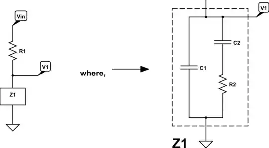
^{simulate this circuit – Schematic created using CircuitLab}

Forget the complicated thing on the right, for now, and just focus on the much simpler thing on the left. Here, we can easily work out that \$V_1=V_\text{IN}\cdot\frac{Z_1}{Z_1+R_1}=\frac{V_\text{IN}}{1+\frac{R_1}{Z_1}}\$. Now, we still don't know how to do much with it. But at least it only requires basic knowledge about voltage dividers. It's kind of abstract, still. But the idea is sound.

Now, we can, in fact work out \$Z_1\$ as being \$Z_{C_1}\$ in parallel with \$Z_{C_2}+R_2\$. In concept, that should also be okay with you, too. Again, the details might be daunting. But at least so far the abstract concepts aren't beyond basic parallel and series impedance ideas. It's just that we know there's some funny stuff in there. But we can worry about that at a later time.

For \$Z_1\$, it's just a parallel combination, so here we can find that \$Z_1=\frac{Z_{C_1}\cdot \left(Z_{C_2}+R_2\right)}{Z_{C_1}+ \left(Z_{C_2}+R_2\right)}=\frac{Z_{C_1}}{1+\frac{Z_{C_1}}{Z_{C_2}+R_2}}\$. Looks messy. But looks right, too.

Separately, you also know that

^{simulate this circuit}

Is just another divider. So we know that \$V_\text{OUT}=V_1\cdot\frac{R_2}{R_2+Z_{C_2}}=\frac{V_1}{1+\frac{Z_{C_2}}{R_2}}\$

We can now combine what we know and get:

$$\begin{align*} V_\text{OUT}&=\frac{\frac{V_\text{IN}}{1+\frac{R_1}{Z_1}}}{1+\frac{Z_{C_2}}{R_2}}\\\\\therefore\\\\ \frac{V_\text{OUT}}{V_\text{IN}}&=\frac{\left[\frac{1}{\left[1+\frac{R_1}{\left[\frac{Z_{C_1}}{1+\frac{Z_{C_1}}{Z_{C_2}+R_2}}\right]}\right]}\right]}{\left[1+\frac{Z_{C_2}}{R_2}\right]} \end{align*}$$

We know that \$Z_{C_1}=\frac1{s\, C_1}\$ and that \$Z_{C_2}=\frac1{s\, C_2}\$. Since in your case \$R_1=R_2=R\$ and \$C_1=C_2=C\$ then:

$$\frac{V_\text{OUT}}{V_\text{IN}}=\frac{\left[\frac{1}{\left[1+\frac{R}{\left[\frac{\frac1{s\, C}}{1+\frac{\frac1{s\, C}}{\frac1{s\, C}+R}}\right]}\right]}\right]}{\left[1+\frac{\frac1{s\, C}}{R}\right]}=\frac{R C s}{\left(R C s\right)^2+3 R C s + 1}$$

Looking at the right side, that's a bandpass filter form (note s with a power of 1 in the numerator but s with a power of 2 in the denominator?) But it's not in standard form. To get it into standard form, let's consider the numerator coefficients to be \$a_i\$ and the coefficients in the denominator to be \$b_i\$, where \$i\$ is the power of \$s\$ that the coefficient is associated with. We then can say: \$a_2=0\$, \$a_1=R C\$, \$a_0=0\$, \$b_2=R^2 C^2\$, \$b_1=3 R C\$, and \$b_0=1\$.

There's two ways to write the standard form for a 2nd order transfer equation for a band-pass filter like this one:

$$\mathcal{T}\left(s\right)=\mathcal{H}\left(s\right)=\mathcal{G}\left(s\right)=K\frac{2\zeta\,\omega_{_0}s}{s^2+2\zeta\,\omega_{_0}s+\omega_{_0}^{\,2}}=K\frac{2\zeta\left(\frac{s}{\omega_{_0}}\right)}{\left(\frac{s}{\omega_{_0}}\right)^2+2\zeta\left(\frac{s}{\omega_{_0}}\right)+1}$$

You need to learn to not just recognize these two forms, but to generate them as well. They both are easy to read. (In a sense, putting an equation into standard form is like taking a circuit and drawing it in a way that is easy to read.) Above, there are just three really important things to note about them:

1. The pole frequency, \$\omega_{_0}\$ or also \$\omega_{_p}\$, which is the angular frequency at which the 2nd order equation does more interesting things; and,
2. The unitless damping factor, \$\zeta\$, which is exactly 1 when the 2nd order equation is critically damped and less than 1 when the 2nd order equation is under-damped and greater than 1 when the 2nd order equation is over-damped. It's also related to the pole quality factor, \$Q\$, where \$Q=\frac1{2\zeta}\$.
3. The gain \$K\$. For low-pass filters this is the gain when well below the pole frequency; for high-pass filters this is the gain when well above the pole frequency; and for band-pass filters (like this one) this is the gain when at the pole frequency.

Everything frequency-related about a 2nd order filter is captured with these three details. You don't need to know anything else about it. (The time domain is a different story, where things such as the peak overshoot might be something else interesting about the filter, as real active filters do have limits on the ranges allowed for their inputs and outputs.)

So to get the above non-standard transfer function into a more standard form, we can set:

$$\begin{align*} \omega_{_0}&=\sqrt{\frac{b_0}{b_2}}=\frac1{R C}\\\\ \zeta&=\frac12\frac{b_1}{\sqrt{b_2 b_0}}=\frac32\\\\ K&=\frac{a_1}{b_1}=\frac13 \end{align*}$$

This is over-damped, as \$\zeta\gt 1\$, and \$20\log_{10}\left(K\right)\approx {-9.54}\:\text{dB}\$ and says that even at the peak this will still attenuate the signal.

---

P.S. The standard forms for a low-pass filter are:

$$\mathcal{T}\left(s\right)=\mathcal{H}\left(s\right)=\mathcal{G}\left(s\right)=K\frac{\omega_{_0}^{\,2}}{s^2+2\zeta\,\omega_{_0}s+\omega_{_0}^{\,2}}=K\frac1{\left(\frac{s}{\omega_{_0}}\right)^2+2\zeta\left(\frac{s}{\omega_{_0}}\right)+1}$$

In the low-pass case, \$K=\frac{a_0}{b_0}\$.

And the standard forms for a high-pass filter are:

$$\mathcal{T}\left(s\right)=\mathcal{H}\left(s\right)=\mathcal{G}\left(s\right)=K\frac{s^2}{s^2+2\zeta\,\omega_{_0}s+\omega_{_0}^{\,2}}=K\frac{\left(\frac{s}{\omega_{_0}}\right)^2}{\left(\frac{s}{\omega_{_0}}\right)^2+2\zeta\left(\frac{s}{\omega_{_0}}\right)+1}$$

In the high-pass case, \$K=\frac{a_2}{b_2}\$.

In all cases, \$\omega_{_0}\$ and \$\zeta\$ are computed as shown, earlier above.

Note that all forms have the same important three constants mentioned earlier.