0

I've been struggling to understand how to get to this expression without knowing about re model (actually, still knowing about it, I can't get to understand this).

In a BJT in, how does one get to Zi = hie+1(1+hfe)RE from the Hybrid Model on an unbypassed emitter configuration?

I saw someone saying it had to do with seeing the resistance from a different terminal it is in, and we had to "move" the (1+hfe) from the current part to the resistance, and this last part is cool to me, I think. Though... I can't understand why we must do this, since I've never done it when calculating the equivalent resistance on a circuit. I also saw it might have to do with having a dependent current source. Though, in my way of viewing this, if Zi is calculated with Vi = 0 V by definition, then the current source evaluates to 0 A and there's no current there --> open circuit, we cut from there and just remains a series of hie with RE (Zi = hie+RE), and that's wrong and I don't get why they're not in series if I just cut the source from there as I always do with the other circuits (the problem might be with the dependent source which I might not be understanding well, but I have no idea).

I've been looking in Electronic Devices and Circuit Theory and in Integrated Electronics Analog and Digital Circuits, but I can't find an explanation of there that comes from without mentioning the re model. If they're equivalent expressions, I'd just like to know how it works, so that they are indeed equivalents not just by the picture but also from the calculus and it would make sense in my head (might also help me understand something I didn't know I didn't understand, as a start).

Bonus: could anyone explain me (or point me to an explanation - that works for the other question too) how to get to that expression, even if from knowing about the re model? Zi = (beta+1)re and Zi = (beta+1)RE --> absolutely no idea how to get to the second from the first one. But maybe that has to do with the first question. Sorry, I'm confused.

Thank you in advance for any help on getting this.

EDIT: maybe I should have mentioned I'm interested not in any hybrid model, but in the h-parameters model. I thought Hybrid Model would lead immediately to h-parameters model (isn't it called only Hybrid Model?).

EDIT 2: I'll accept Verbal Kint's as it is the one that helped me understand the dependent sources (or at least a bit more than I did) with help of a friend removing some wrong ideas (or at least that didn't make sense for me) I had been put in my mind by other people. Though, LvW's answer helped too in understanding a bit better first how to deal with this without going to any models, so thank you both, and I'll accept the one I said because it's the one I'll use more, possibly (we haven't learned much about Control Theory yet, so I didn't completely understand but with time I will). Also sorry, don't have enough reputation, but I hope the 3 people get the upvote I sent. Even though analogsystemsrf's answer didn't help me on what I needed, helped clear something else on my mind so also thank you for that. This is a big text...
Edw590
  • 288
  • 2
  • 9
  • You can start with the [***non-linear*** full-scale Ebers-Moll models](https://electronics.stackexchange.com/a/252199/38098) for the BJT (these are so-called "level 1" and only include a simplified DC model.) With level 2, 1st order modeling of charge storage and a more accurate DC model is given. (Not shown there.) And with level 3, you get base-width modulation (Early Effect and \$r_o\$), a rise of \$\tau_F\$ at higher currents, variation of device pars with temp, and capacitance splitting, to name a few things. The linearized version uses differential equations about a DC operating point. – jonk May 26 '20 at 02:34
  • So keep in mind that when someone talks about the hybrid-\$\pi\$ model, they are usually talking about the ***linearized*** version of it around a DC operating point, derived using differentials and algebraic substitution to get it. They usually are ***not*** talking about the non-linear version which was developed originally by Ebers and Moll's papers on the topic in the 1950's. The above link provides all three ***equivalent*** models that were developed from various ideas: *transport*, *injection*, and *hybrid-* \$\pi\$. These are still the same thing written in different mathematical ways. – jonk May 26 '20 at 02:40
  • The hybrid-\$\pi\$ model chooses to replace the two current sources found, for example, in the transport model into a single current source from collector to emitter. Everything else was then changed, as needed, to still be equivalent. The advantage here is that a linearized, differential form is then much easier to develop. This is why the hybrid-\$\pi\$ model took over and the transport and injection models are now long forgotten. – jonk May 26 '20 at 02:46
  • Thank you. As that's a book and I'm short on time, I won't have time to read it. Though, I'll put it on the list to see at least parts of it. I had no idea about the first 2 models you talk about on the post you linked. Actually never heard of them. Only the third one (hybrid-pi). Interesting. – Edw590 May 26 '20 at 22:52
  • What I wrote at that link is not a book. It's just a quick summary of what I learned from books. Most people today haven't heard of the transport or injection models, but they are more "physical" and therefore "sing better" in the minds of physicists. The hybrid-\$\pi\$ model was created as an equivalent mathematical model which is less physical but easier to teach to non-physicists and easier for everyone to understand how to linearize. And I'm glad Verbal Kint is helping you... – jonk May 27 '20 at 00:16
  • Oh my bad, I meant the book you say in your post. The one from Tektronix, from where you took parts of your post (which I read entirely). Though, I'd like to read parts of the book too because it might be helpful too (and at least interesting to know). – Edw590 May 27 '20 at 10:05
  • That book provides a unique reference, in my opinion. Half of it exists to be a full compendium on the BJT models and meaning, up through Gummel-Poon. Half exists to help you know how to measure those parameters on a bench. I recently met Ian (the author) at the funeral of another Tektronix employee, Barrie Gilbert (of the Gilbert cell fame, for example.) Worth getting and reading, if you are interested in a thorough text on BJTs for engineers. Most folks aren't, as discrete BJT use has waned almost to nothing. – jonk May 27 '20 at 16:55

3 Answers3

2

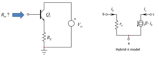
To determine the input resistance of a simple common-collector configuration you have to replace the transistor symbol by its equivalent hybrid-\$\pi\$ model. The common-collector configuration is shown below and the transistor simplified linear model is in the right-side of the picture:

enter image description here

Then, to determine an input impedance or resistance, you install a current source \$I_T\$ (the stimulus) biasing the terminals across which you want the resistance and you express the voltage \$V_T\$ (the response) that it generates. Then, you simply write \$R_{in}=\frac{V_T}{I_T}\$. Here we go with the drawing:

enter image description here

This is a small-signal model in which we consider the \$V_{cc}\$ rail perfectly decoupled meaning that any modulation applied to the circuit won't make the voltage of this rail move. In other words, its differentiation with respect to time is 0, hence the replacement of the source by a wire. To determine the voltage \$V_T\$, we stack the voltage across \$r_\pi\$ with that across the emitter resistance \$R_E\$. In this drawing, the base current is actually the injected current \$I_T\$. Therefore, \$V_T=i_br_\pi+(\beta i_b +i_b)R_E=i_b(r_\pi+(\beta+1)R_E)=I_T(r_\pi+(\beta+1)R_E)\$.

Now, divide \$V_T\$ by \$I_T\$ and you have \$R_{in}=r_\pi+(\beta+1)R_E\$.

Verbal Kint
  • 20,420
  • 1
  • 16
  • 50
  • Hi. Actually, it made sense to me now. But I have another question now, if you wouldn't mind. Isn't the input impedance calculated with that VT equalling 0? Like, Zi, Vi = 0; Zo, Vo != 0 (open circuit though). I can't find where that's written in some book about how to calculate the input and output impedances of a circuit, but isn't the input one calculated with the voltage across the input terminals as 0 V and the output impedance with the output terminals in open circuit? – Edw590 May 26 '20 at 22:50
  • Hi, \$V_T\$ is the response generated by the stimulus \$I_T\$. This response could be 0 V if a zero was present and we were to determine an input impedance. But in this dc application, \$V_T\$ is well alive. Same with the output impedance determination across \$R_E\$. If you are interested by determining transfer functions and the associated analyses techniques, you can find more details in the [book](https://www.amazon.com/Linear-Circuit-Transfer-Functions-Introduction/dp/1119236371/ref=la_B001IOH604_1_3?s=books&ie=UTF8&qid=1461931295&sr=1-3) I wrote on the subject. – Verbal Kint May 27 '20 at 07:30
  • A question (going out of the main question). If I wanted to calculate the input impedance by starting with rpi // RE, do you know how I could still get to the correct result? Or there's no way because of the dependent source? (I don't know the internal resistance of those sources - or if it has nothing to do with that, I don't know how one would put the resistances in paralell as a start and then get to the correct result. Is that possible to do? – Edw590 May 27 '20 at 15:52
  • Why do you focus on the paralleling of the two resistances? I don't see how this could be done in this simple analysis. – Verbal Kint May 27 '20 at 16:53
  • A friend of mine looked at it and started by saying they were both in parallel. So I was wondering if it could be done that way. Thank you. But I did wanted the series explanation as you did. The parallel was just a curiosity. – Edw590 May 27 '20 at 18:47
0

As jonk suggests in his profile, a fully-detailed example can be useful to understanding.

Here is a partially detailed example.

  • when the emitter current is varied, and let us use tiny variations such as 1% or evev 0.1% variations so the exponential_diode_I_V curve is "linear", we can describe the resistance ( delta_Vdiode / delta_Idiode ) as 0.026 volts / Idiode_amperes. Thus operating at 0.001 amp produces 0.026 / 0.001 == 26 ohms. I've used that value ----- 26 ohms at 1milliAmp ----- for decades happily in my bipolar voyages. Knowing that is key to almost trivial back_of_envelope circuit design.

  • we are in a system where injected base current attracts opposing carriers from the emitter, and most of the emitted charges MISS the base charges and rush on across the base region to be gathered up in the collector. The ratio of base_charges to emitter_charges is huge, and is described by some variant of BETA.

  • the base current is assisted by beta_multiplication to become the emitter current

  • input_resistance math becomes: beta * ( 0.026 volts / Iemitter_amperes )

  • for a bipolar operating at 1 milliamp Iemitter, with beta of 200, the input resistance == 200 * 26 = 5,200 ohms

analogsystemsrf
  • 33,703
  • 2
  • 18
  • 46
0

Here comes my (very short) answer:

From system theory we know that the input impedance of a circuit with feedback (if the feedback signal is a voltage) will be enlarged by the factor (1-loop gain). The same expression appears in the closed loop gain where it appears in the denominator (the gain is reduced by this factor).

As it is shown in the figure below, the gain around the feedback loop (loop gain) is LG=-gm * RE.

Hence, Zi=hie * (1+ gm * RE) with gm=hfe/hie, we arrive at

Zi=hie + hfe * Re.

(In this formula, we have hfe instead of (1+hfe) because I have assumed, for simplicity, Ie=Ic. The difference between hfe and (1+hfe) can be neglected).

Remark: I know that - primarily - you are interested in a derivation of that formula from the Pi-model. However, for my opinion, it is always interesting to get a confirmation based on a complete other approach - for example from the viewpoint of system theory.

UPDATE/EDIT: I do not like and I do not need transistor models. Instead, it is very simple to derive the formula for the input resistance using basic formulas:

h11=vbe/ib=vb/ib-ve/ib.

With ve=RE * ie =RE(1+h21)ib we immediately arrive at

ri=vb/ib=h11+ve/ib=h11+RE(1+h21)

enter image description here

LvW
  • 24,857
  • 2
  • 23
  • 52
  • Hi. Your answer is the one that gets the most near to what I wanted to know the most (how to get to the formula using the h-parameters) --> I'm actually interested in the h-parameter model haha. I've just put that in an EDIT. I thought Hybrid Model would lead immediately to h-parameter model, not to Hybrid-pi. My bad, I didn't know. – Edw590 May 26 '20 at 14:51
  • h-parameters are based on the two-port network theory. In short $$ h_{ie} = h_{11} \approx r_\pi , h_{fe} = h_{21} \approx \beta , h_{oe} =h_{22} \approx \frac{1}{r_o}$$ – G36 May 26 '20 at 15:03