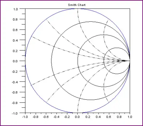
I wrote a gnuplot script that generates Smith Charts. The circles are a little sparse, but you can add more if needed. If you want to get really wild and crazy, there are even routines to draw circular arcs along constant X or constant R circles so you add more gridlines on part of the chart, or make the "grid circles" less dense in places. I also included some funcitons for annotating impedance (and admittance) on the charts.
Here is the script...
# Smith Chart Plotting Tools
# Written By: Jess Stuart  4/21/2020
# Tested with gnuplot 5.2 patchlevel 6

reset
# Control Variables
chartType = 1  # 0=blank, 1=impedance, 2=admittance, 3=immitance
ZAxisLabels = 1  # controls if axis labels are printed or not. 1=true, 0=false.
YAxisLabels = 1  # controls if axis labels are printed or not. 1=true, 0=false.

set clip points
set parametric # t is gnuplot's default single parametric variable
set samples 500 # affects circle smoothness
unset key
set style increment default
set size ratio 1 1,1
set style data lines
unset border
set trange [0:pi/2] noreverse nowriteback  # tan(t) goes from 0 to +inf
set xrange [-1.1:1.1] noreverse nowriteback
set yrange [-1.1:1.1] noreverse nowriteback
unset xtics
unset ytics

# Linear Map t to something else
LM(t,S,E)=2*(E-S)*t/pi + S  # t goes from 0 to pi/2
# Pertibation Function (causes parametric plot to draw a point without using a         "point"; useful for debugging)
e(t)= t*{0.002,0.002}
# Evaluate String Expressions!!!
# usage:
# 1. store value to t. (Ex. t=0.5)
# 2. eval(wrapper(strExp)) assigns outVal the value of the string expression     evaluated at t.
# 3. use outVal in whatever calculation you wanted (Ex. setting label text)
wrapper(strExp)=sprintf("outVal=%s",strExp)

# Simplify parametric plotting on the complex plane. Must use eval() on returned string.
plot_complex(s,a) = sprintf("plot real(%s),imag(%s) %s",s,s,a)
replot_complex(s,a)= sprintf("replot real(%s),imag(%s) %s",s,s,a)

#constant value circle plotting
conValCirs(i,Start,End,s,a) = sprintf("replot for [%s=%d:%d] real(%s),imag(%s) %s",i,Start,End,s,s,a)

# Complex Parametric Circle Function
CIRCLE(t,r,xc,yc)=r*(cos(t)+{0,1}*sin(t)) + xc + {0,1}*yc

#"set angles degrees" will mess up tan(t) used to draw the constant R, constant X circles
# Use these functions to convert from degrees to radians or plot polar data that uses
# angles in degrees.
DEG2RAD(d)= d*pi/180
POL2X(r,d)=r*cos(d*pi/180)
POL2Y(r,d)=r*sin(d*pi/180)

# Complex Reflection Coefficient Functions
Z2RC(z)=((z)-1)/((z)+1) #impedance to reflection coefficient
Y2RC(y)=(1-(y))/((y)+1) #admittance to reflection coefficient
sZ2RC(z)=sprintf("((%s)-1)/((%s)+1)",z,z) # string version
sY2RC(y)=sprintf("(1-(%s))/((%s)+1)",y,y) # string version

# Constant Resistance or Reactance Circular Arc Functions
RARC(t,R,X1,X2,a)=sprintf("replot real(Z2RC(t*(%s)/t+{0,1}*LM(t,%s,%s))),imag(Z2RC(t*(%s)/t+{0,1}*LM(t,%s,%s))) %s",R,X1,X2,R,X1,X2,a)
XARC(t,X,R1,R2,a)=sprintf("replot real(Z2RC(LM(t,%s,%s)+{0,1}*t*(%s)/t)),imag(Z2RC(LM(t,%s,%s)+{0,1}*t*(%s)/t)) %s",R1,R2,X,R1,R2,X,a)
GARC(t,G,B1,B2,a)=sprintf("replot real(Y2RC(t*(%s)/t+{0,1}*LM(t,%s,%s))),imag(Y2RC(t*(%s)/t+{0,1}*LM(t,%s,%s))) %s",G,B1,B2,G,B1,B2,a)
BARC(t,B,G1,G2,a)=sprintf("replot real(Y2RC(LM(t,%s,%s)+{0,1}*t*(%s)/t)),imag(Y2RC(LM(t,%s,%s)+{0,1}*t*(%s)/t)) %s",G1,G2,B,G1,G2,B,a)

# Combine an impedance(admittance) with a parallel(series) admittance(impedance).      Returns a calculation string for impedance(admittance).
INVADDINV(A,B)=sprintf("1/(1/(%s)+(%s))",A,B)

# convert impedance(admittance) to admittance(impedance)
FLIP(U)=sprintf("t*1.0/((%s)*t)",U)

# Calculate radius of a SWR circle
SWR2RADIUS(swr)=(swr-1)/(swr+1)

# Constant Circle Values: Array length must match indexing variable range in plot statements

# Impedance Chart
array Xvals[17] = [-10.0,-5.0,-2.5,-1.5,-1.0,-0.7,-0.4,-0.2,\
                     0.0,\
                    10.0, 5.0, 2.5, 1.5, 1.0, 0.7, 0.4, 0.2,]
array Rvals[7] = [0.0,0.2,0.5,1.0,2.0,4.0,10.0]
# Admittance Chart
array Bvals[17] = [-10.0,-5.0,-2.5,-1.5,-1.0,-0.7,-0.4,-0.2,\
                     0.0,\
                    10.0, 5.0, 2.5, 1.5, 1.0, 0.7, 0.4, 0.2,]
array Gvals[7] = [0.0,0.2,0.5,1.0,2.0,4.0,10.0]

# Styles used for plots
set style line 1 lw 1 lc rgb "black"  # Impedance (Z)
set style line 2 lw 1 lc rgb "red"  # Admittance (Y)
set style line 3 lw 1 lc rgb "#008000" # dark green
set style line 4 lw 2 lc rgb "blue" #use for ploting frequency response
set style line 5 lw 2 lc rgb "magenta" # second frequency response
set style line 6 lw 2 lc rgb "cyan" # third frequency response

# Axis labels on Smith Chart
XCIR_LABEL(X,a)=sprintf("set label \"%.1f\" at %f,%f %s", X, 1.05*(X*X-1)/(X*X+1),1.05*2*X/(X*X+1),a )
RCIR_LABEL(R,a)=sprintf("set label \"%.1f\" at %f,%f %s", R, (R-1)/(R+1),0.05,a)
BCIR_LABEL(B,a)=sprintf("set label \"%.1f\" at %f,%f %s", B, -1.05*(B*B-1)/(B*B+1),-1.05*2*B/(B*B+1),a )
GCIR_LABEL(G,a)=sprintf("set label \"%.1f\" at %f,%f %s", G, -(G-1)/(G+1),0.05,a)

# Useful for Annotating Plots.
Z_MARKER(indx,Z,str,a) = sprintf("set label %s \"z=%.2f%sj%.2f\ %s\" at %f,%f point ls 1 pt 5 offset 0.4,-0.4 tc ls 1 %s",\
                        indx, real(Z),((sgn(imag(Z))==1)?"+":"-"),abs(imag(Z)),\
                        str, real(((Z)-1)/((Z)+1)),imag(((Z)-1)/((Z)+1)),a)
Y_MARKER(indx,Y,str,a) = sprintf("set label %s \"y=%.2f%sj%.2f\ %s\" at %f,%f point ls 2 pt 5 offset 0.4,-0.4 tc ls 2 %s",\
                indx, real(Y),((sgn(imag(Y))==1)?"+":"-"),abs(imag(Y)),\
                str, real((1-(Y))/(1+(Y))),imag((1-(Y))/(1+(Y))),a)
RC_MARKER(indx,S,str,a)= sprintf("set label %s \"{/Symbol G}=%.2f%sj%.2f\ %s\" at %f,%f point ls 3 pt 5 offset 0.4,-0.4 tc ls 3 %s",\
                indx, real(S),((sgn(imag(S))==1)?"+":"-"),abs(imag(S)),\
                str, real(S),imag(S),a)
TEXT_LABEL(indx,S,str,a) = sprintf("set label %s \"%s\" at real(%s),imag(%s) %s",indx,str,S,S,a) # plot text on the complex-plane

if (chartType==0){
    set title "Blank Smith Chart" tc rgb "gray"
}
if (chartType==1){
set title "Normalized Impedance Smith Chart" tc ls 1
}
if (chartType==2){
    set title "Normalized Admittance Smith Chart" tc ls 2
}
if (chartType==3){
    set title "Normalized Immitance Smith Chart" black
}

plot 0,0 black  # create a plot to get started
# Blank (Useful for debugging plotting commands)
if (chartType==0) {
    eval(replot_complex("CIRCLE(4*t,1,0,0)","black"))
}
# Impedance Chart Part
if ((chartType==1) || (chartType==3)) {
    eval(conValCirs("i",1,|Rvals|,"Z2RC(Rvals[i]+{0,1}*tan(2*t))","ls 1"))     #tan(2t) => 0 to +inf to -inf to 0
    eval(conValCirs("i",1,|Xvals|,"Z2RC(tan(t)+{0,1}*Xvals[i])","ls 1"))
    # Labels
    if (ZAxisLabels!=0){
        do for [i=1:|Rvals|] {
         eval(RCIR_LABEL(Rvals[i],"center tc rgb \"black\""))
         }
        do for [i=1:|Xvals|] {
        eval(XCIR_LABEL(Xvals[i],"center tc rgb \"black\""))
        }
    }
}
# Admittance Chart Part
if ((chartType==2) || (chartType==3)) {
    eval(conValCirs("i",1,|Gvals|,"Y2RC(Gvals[i]+{0,1}*tan(2*t))","ls 2")) # tan(2t) 0 to +inf to -inf to 0
    eval(conValCirs("i",1,|Bvals|,"Y2RC(tan(t)+{0,1}*Bvals[i])","ls 2"))
    # Labels
    if (YAxisLabels!=0){
        do for [i=1:|Gvals|] {
        eval(GCIR_LABEL(Gvals[i],"center tc rgb \"red\""))
        }
        do for [i=1:|Bvals|] {
        eval(BCIR_LABEL(Bvals[i],"center tc rgb \"red\""))
        }
    }
}
if ((chartType!=0) && (chartType!=1) && (chartType!=2) && (chartType!=3)) {
    print("Unknown chartType.")
 }
#########################################
###### PLOT DATA HERE WITH REPLOT ######

# replot...
refresh #draw the labels
############################################
############################################
## Ex. Constant SWR Circle
#eval(replot_complex("CIRCLE(4*t,SWR2RADIUS(3.0),0,0)","ls 3"))
#############################################
#############################################
##Ex. Parallel RLC circut impedance
#Z0=50 #Characteristic Impedance
#f1=1e7
#w1=2*pi*f1
#f2=1e9
#w2=2*pi*f2
#R1(t)=t*40/t  # 32 ohm, "Vectorize" R by multiplying and dividing by parameter t.
#C1=3.3e-11 # 33 pF
#L1=1.8e-7 # 180 nH
#Y1(t)=Z0*(1/R1(t) + {0,1}*(LM(t,w1,w2)*C1 - 1/(LM(t,w1,w2)*L1) ) ) #Normalized
#eval(replot_complex("Y2RC(Y1(t))","ls 4"))
#R2(t)=t*60/t  # 32 ohm, "Vectorize" R by multiplying and dividing by parameter t.
#C2=8.0e-11 # 80 pF
#L2=2.7e-7 # 180 nH
#Y2(t)=Z0*(1/R2(t) + {0,1}*(LM(t,w1,w2)*C2 - 1/(LM(t,w1,w2)*L2) ) ) #Normalized
#eval(replot_complex("Y2RC(Y2(t))","ls 5"))
##############################################
##############################################
##Ex. Impedance Matching Network Smith-Chart Trajectories
#Cc=10e-12 # 10pF
#Ls=4.2e-9 #6nH
#Cp=4.7e-12 #4.7pF
##50 ohm characteristic impedance (adjust constants as necessary)
## helper functions with constants combined (needs parameter t)
## Build up Nested string expressions (to create a self-contained demo).
## Use a program to write columns to a datafile, then plot the
## data with gnuplot; Nested calculations inside gnuplot are cumbersome!
#Xc(f,C)=sprintf("t*{0,-0.00318310}/((%e)*(%e)*t)",f,C)  # -1/(2*pi*50)
#Xl(f,L)=sprintf("t*{0, 0.125664}*(%e)*(%e)/t",f,L) # 2*pi/50
#Bc(f,C)=sprintf("t*{0, 314.159}*(%e)*(%e)/t",f,C) # 2*pi*50
#Bl(f,L)=sprintf("t*{0,-7.95775}/(%e)*(%e)*t)",f,L) # -50/(2*pi)
#array freqs[3]=[1.70e9, 1.75e9, 1.80e9]
#do for[j=1:|freqs|] {
#    Yload=sprintf("t*50/(160*t)+(%s)",Bc(freqs[j],3e-12)) # load = (160ohm || 3pF)
#    Zload=FLIP(Yload)
#    Z1=sprintf("(%s)+(%s)", Zload, Xl(freqs[j],Ls)) #add series inductance
#    Y1=FLIP(Z1)  # used to plot constant conductance curve
#    Z2=INVADDINV(Z1,Bc(freqs[j],Cp)) # add shunt capacitance
#    Y2=FLIP(Z2)
#    Z3=sprintf("(%s)+(%s)", Z2, Xc(freqs[j],Cc)) # add series capitance   (coupling)
#    eval(RARC(t,"real(".Zload.")","imag(".Zload.")","imag(".Z1.")",sprintf("lw 3 lc %d",j)))
#    eval(GARC(t,"real(".Y1.")","imag(".Y1.")","imag(".Y2.")",sprintf("lw 3 lc %d",j)))
#    eval(RARC(t,"real(".Z2.")","imag(".Z2.")","imag(".Z3.")",sprintf("lw 3 lc %d",j)))
#    t=pi/2 #end value of sweep
#    eval(wrapper(Z3)) # evaluates at t, and assigns value to outVal.
#    eval(Z_MARKER("",outVal,"",""))
# }  #loop
#refresh #draws last label
#######################################################
#######################################################
## label tests
#eval(Z_MARKER("",{0,0},"",""))
#eval(Y_MARKER("",{0,0},"",""))
#eval(RC_MARKER("",{0,0},"",""))
#eval(TEXT_LABEL("","{-0.24,0.77}","test","point ls 4 pt 5 offset 0.4,0.4 tc ls 4 "))
#refresh
#######################################################