This type of configuration is always intimidating considering the weird op-amps arrangement. To look at the impedance, I prefer using the fast analytical circuits techniques or FACTs described in the book I wrote. To determine an impedance, you can install a test generator \$I_T\$ producing a voltage \$V_T\$ across its terminals. the ratio \$\frac{V_T}{I_T}\$ is the impedance you want.
First, I check the basic dc resistance \$R_0\$ with the complete circuit and a re-drawn version implying non-ideal op-amps. Running an operating point SPICE simulation tells me if I'm good to go. Bias points say yes:
To determine the dc input resistance \$R_0\$, open the capacitor and determine \$R_0=\frac{V_T}{I_T}\$ in this mode:
With a few equations, you confirm the dc operating points:
In the above lines, you see that with an open-loop gain approaching infinity, the dc resistance is 0 \$\Omega\$.
The next step is to determine the pole position. Turn the excitation off (zero the current source) and install the test generator across the capacitor:
If you do the maths ok, you find:

With a gain approaching infinity, the pole is infinite too. Now, for the zero, you have to null the response. The response is \$V_T\$ across the current source in the first sketch. When nulled, we have a degenerate case and the current source can be replaced by a short circuit. Determine the resistance seen from the capacitor connecting terminals in this mode and you have the zero position:
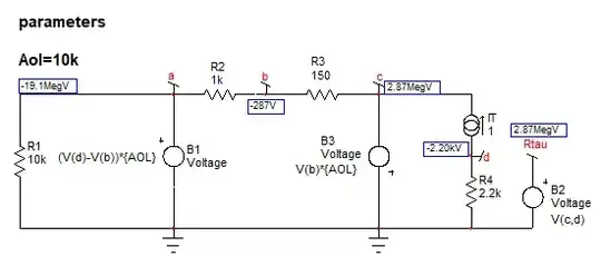
Again, if the maths are ok you have:
This is it, we have the complete impedance transfer function expressed as:
\$Z_{in}=R_0\frac{1+\frac{s}{\omega_z}}{1+\frac{s}{\omega_p}}\$. From this formula, considering an inductive impedance equal to \$Z_L=R_0+sL_{eq}\$, we can express the emulated inductance equal to: \$L_{eq}=\frac{R_0}{\omega_z}\$:
With the component values I used, the inductance is 330 µH with a 1.5-\$\Omega\$ dc resistance in series. If the op-amps are perfect, you have a purely inductive component. The input impedance plot with a 10k open-loop gain is there:
Here the FACTs let you determine the complete transfer function without analyzing the circuit: determine the time constants in two conditions (zeroed excitation and nulled response) and you have your transfer function including the op-amp open-loop gain effects. What is cool is that you can use SPICE to check your calculations via a .OP simulation and make sure the bias points exactly match the Mathcad sheet. This is an excellent way to progress in the process without making mistakes.


