Dominant Pole Approximation

Question

I am studying Microelectronics by Behzad Razavi, 2nd Ed., where in the frequency response chapter it uses the "Dominant Pole Approximation" to find one of the poles easily from a quadratic denominator in the transfer function (he did this as the coefficients involved were HUGE.. it was a calculation involving the high frequency response of a MOS common source amplifier).

Is the this approximation used only to simplify calculations? What intuition can we gain from such an approximation?

He did not include any bode plot with this particular analysis.

Answer 1

Your circuit features 3 capacitors but is actually a 2nd-order system (degenerate case). The denominator of the transfer function (whatever it is) follows the following formalized form: \$D(s)=1+\frac{s}{\omega_0Q}+(\frac{s}{\omega_0})^2\$.

In this expression, \$Q\$ represents the quality factor and illustrates the losses in your circuit. Because \$D(s)\$ is a 2nd-order expression, there are two roots or poles. Depending on the value of \$Q\$, we can distinguish three scenarii:

1. \$Q\$ is large, greater than 0.5: the poles are complex conjugate, the time-domain response is a damped oscillatory waveform.

2. \$Q\$ is equal to 0.5: the poles are coincident, the roots are real (no imaginary term) and the response to a step input is fast, without oscillations.

3. \$Q\$ is small, much lower than 0.5, e.g. 0.01 for instance: the poles are real and well spread from each other. In this case, the denominator can be approximated - hence the term associated with this arrangement: the low-\$Q\$ approximation - to two cascaded poles: \$D(s)=1+\frac{s}{\omega_0Q}+(\frac{s}{\omega_0})^2\approx (1+\frac{s}{\omega_{p1}})(1+\frac{s}{\omega_{p2}}) \$. In this mode, it is easy to show that \$\omega_{p1}=Q\omega_0\$ and \$\omega_{p2}=\frac{\omega_0}{Q}\$. If \$Q\$ is really small, then you naturally see that \$\omega_{p1}\$ is lower and dominates the low-frequency response while \$\omega_{p2}\$ is higher and can be neglected provided the high-frequency response is of lesser interest.

If I had to analyze this circuit, I would recommend the usage of the fast analytical circuits techniques or FACTs which will let you obtain a low-entropy transfer function in a flashing time.

Answer 2

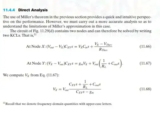
The circuit presented in your figure is a full hybrid-pi model, using that model it is possible to find the output of the MOSFET at the drain for a given input. That relation, in a linear circuit, can be represented as a transfer function, which will make all the terms that depend on derivatives and integrals of time become either \$ s \$ (for derivatives) or \$ \frac{1}{s} \$ for integrals (instead of calculus you can use algebra for the output/input relation).

With all the parameter in the model and using KCL he rearranges the equation for node Y into isolating \$V_X\$, which he substitute in the equation for node X, giving a equation with \$V_{out}\$ and \$V_{Thev}\$ (his input to the gate). He then rearenges the formula from 11.69 to 11.70, but, to avoid a huge formula he separates the terms for the characteristic equation. The roots of this equation are the poles of your system, and they give you the modes for it (the responses you can get from a pulse, impulse, sine and so on).

The trick or "insight" the author gives is representing the characteristic equation as the product of its roots (poles) and then supposing one of the poles is ways smaller than the other \$\omega_{p_2} << \omega_{p_1}\$. That being said the term \$b\$ is used as approximate to this large pole \$ \omega_{p_1}\$.

The reason for approximating this pole, and not bother finding the other, must be that the other occurs at very high frequencies (I suppose >100 kHz), while this larger pole occurs in the range of frequencies that the MOSFET is supposed to operate.