This might be of interest to you. It demonstrates how to empirically find the 3 most useful diode parameters: saturation current (IS), series resistance (RS), and the emission coefficient (N).
There's quite a bit of mathematical background at the beginning, but for the most part you can skip this (unless you are interested in the math).
At the end, I include some Python code which can be used to calculate these three parameters either from a datasheet I-V graph or experimental measurements.
You will also need to know the reference temperature (what temperature your measurements are at, or what temperature the I-V graph is for), as well as roughly what temperature you intend to run the device at (typically 298K is a good default choice, though many datasheets specify at 293K).
To easily get accurate data from an I-V graph, try using a plot digitizer.
For pretty much everything else, you can use the "standard" values unless you have some specific requirements (notably time dependent and more accurate temperature dependent effects).
For future reference, here's a stripped down (i.e. comments removed) version of the code:
from numpy import *
from scipy.optimize import leastsq

def diode_res(args, T, V, I):
    n, Rs, Is = args
    kb = 8.617332478e-5
    return I*Rs+log(I/Is+1)*n*kb*T-V

def jac_diode(args, T, V, I):
    n,Rs,Is = args

    kb = 8.617332478e-5
    res = zeros([3,len(V)])
    res[0,:] = log(I/Is+1)*kb*T
    res[1,:] = I
    res[2,:] = -I/(I*Is+Is**2)*n*kb*T
    return res

def diode_coeffs(V, I, T):
    return leastsq(diode_res, array([1,0,1e-14]),args=(T,V,I), Dfun=jac_diode, col_deriv=True,xtol=1e-15)[0]
It works by performing a non-linear least squares fit. Here's an example usage (I grabbed data from the I-V plot in your link):
I = array([0.00139106,  0.00186955,  0.00258687,  0.00210901,  0.00324447, 0.00282632,  0.00372254,  0.0063513 ,  0.00724731,  0.00676945, 0.00820303,  0.00772517,  0.0086809 ,  0.01178709,  0.01278269, 0.01226495,  0.0134595 ,  0.0168444 ,  0.01632666,  0.01799907, 0.01752121,  0.01847693,  0.02134388,  0.02086602,  0.02235931])])
V = array([ 3.04213083,  3.10179528,  3.16154354,  3.14650173,  3.22127085, 3.20624999,  3.25118688,  3.37110238,  3.40116506,  3.38612324, 3.43124868,  3.41620687,  3.44629049,  3.55149938,  3.58655504, 3.56654119,  3.59670861,  3.70697334,  3.68695949,  3.73216872, 3.71712691,  3.74721053,  3.82258719,  3.80754538,  3.85269177])

# assume data is at 20C
n, Rs, Is = diode_coeffs(V, I, 273+20)
Results:
- n = 5.5287
- Rs = 18.983 \$\Omega\$
- Is = 0.506623 pA
Here's a plot with the fit parameters:
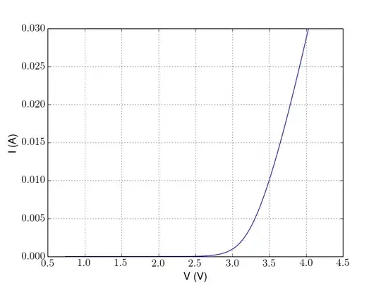
Here is the resulting I-V curve from LtSpice, using only these three parameters and everything else the default diode values. As you can see, there is some slight mismatch, but in general this is usually within actual part noise (i.e. you shouldn't rely on getting exactly 30mA at 4V, 27mA is not unreasonable).